

Pendahuluan
“Cheapest machine” often turns into the most expensive line after year two. Energy spikes, scrap drift, and downtime eat margins fast. In this guide, I show a simple, practical way to model Total Cost of Ownership (TCO) for an extrusion blow molding machine—so you judge by cost per good bottle, not sticker price. You’ll map the big cost buckets, pressure-test key assumptions, and compare two machines apples-to-apples. Short, clear steps. Actionable checks. Use it before the next RFQ.
What You’ll Need
Last 12 months’ run hours, SKU mix, scrap %, and good bottles/hour per SKU.
Local electricity tariff and demand charges; compressed air and chiller specs.
Resin price range (virgin HDPE, rHDPE/PCR), typical gram weights.
Maintenance logs: planned/unplanned stops, parts spend, MTTR.
Quotes for machines, tooling, auxiliaries, installation, and layanan terms.
Define Scope and Time Horizon

Pick a clear window: 5–10 years is enough to cover one or two major upgrades and show total cost, not just the purchase price. Shorter than 5 years hides maintenance and energy costs. Longer than 10 years gets fuzzy because product lines, materials, and labor rules change.
Actions
Choose a time horizon: 5, 7, or 10 years. Keep it consistent across options.
List SKUs you’ll run: sizes, resins (like HDPE or PET), and bottle/jerry can families. Note annual volume and seasonality.
Define shifts: 1–3 shifts per day, days per week, planned uptime, and maintenance stops. Convert that into annual available hours.
Estimate growth: base case, conservative, and stretch. Tie growth to real triggers like a new customer contract or recycled material requirements.
Avoid
Don’t compare “cycle time” across machines without SKU mix and changeover rules. A fast cycle on paper can lose in real life if changeovers are frequent, scrap spikes on certain resins, or the mold set is limited.
Tools
Use one spreadsheet with three tabs:
Assumptions: time horizon, SKUs, shifts, uptime, growth, resin type.
Costs: CapEx, molds, utilities, labor per shift, maintenance, spare parts, training.
Results: output per year, cost per bottle, total cost of ownership, sensitivity cases.
Hasil
You end up with a clean boundary: what’s inside the model and what’s not. That keeps debates focused on inputs, not opinions.
Visual
Show one simple timeline: CapEx in Year 0, then OpEx bars (energy, labor, maintenance) for each year. Add markers where growth or SKU changes kick in.
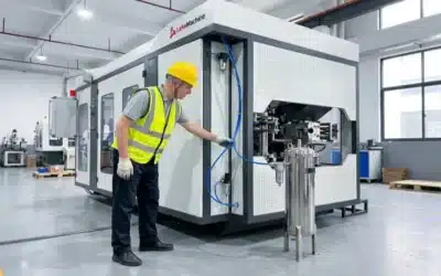
Capture CapEx and Tooling
Build the CapEx list from the clamp to the conveyor. The goal is a true “landed” cost, not just the base machine. Keep it simple, but complete.
Actions
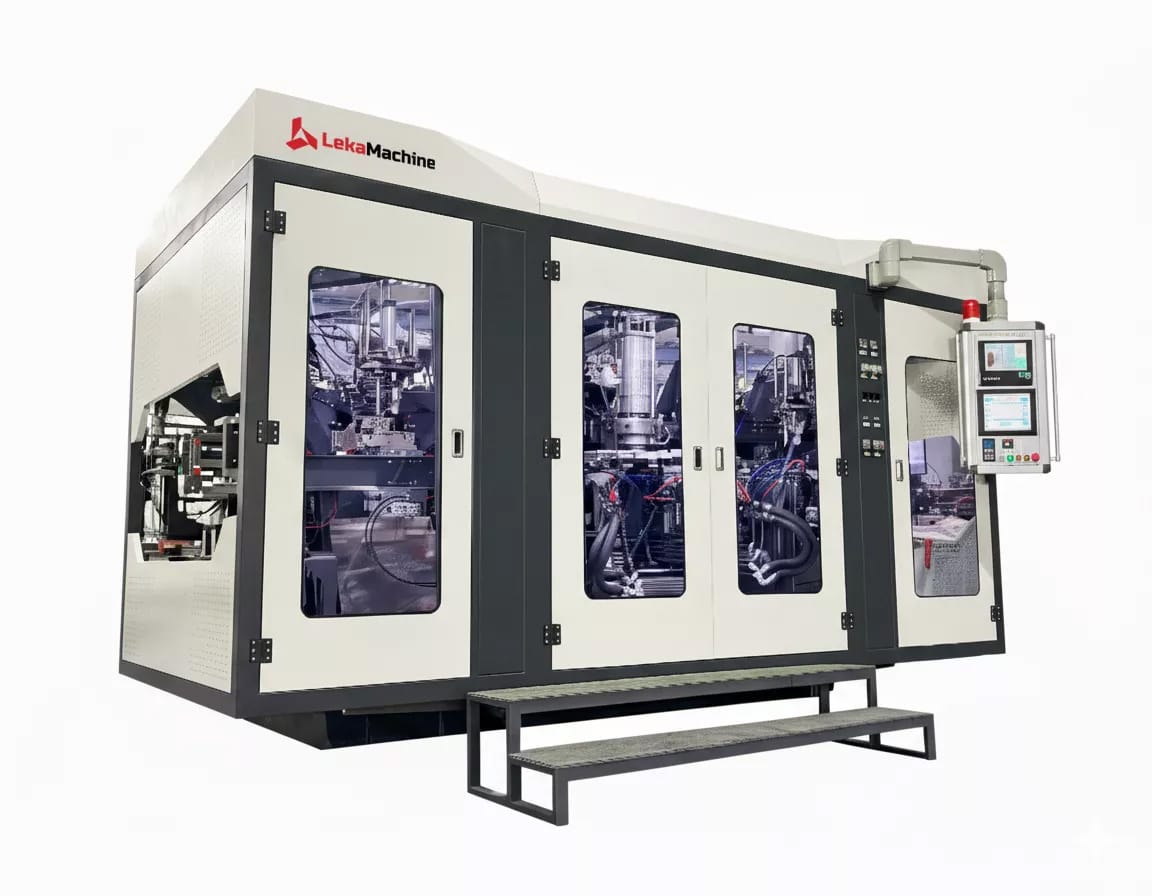
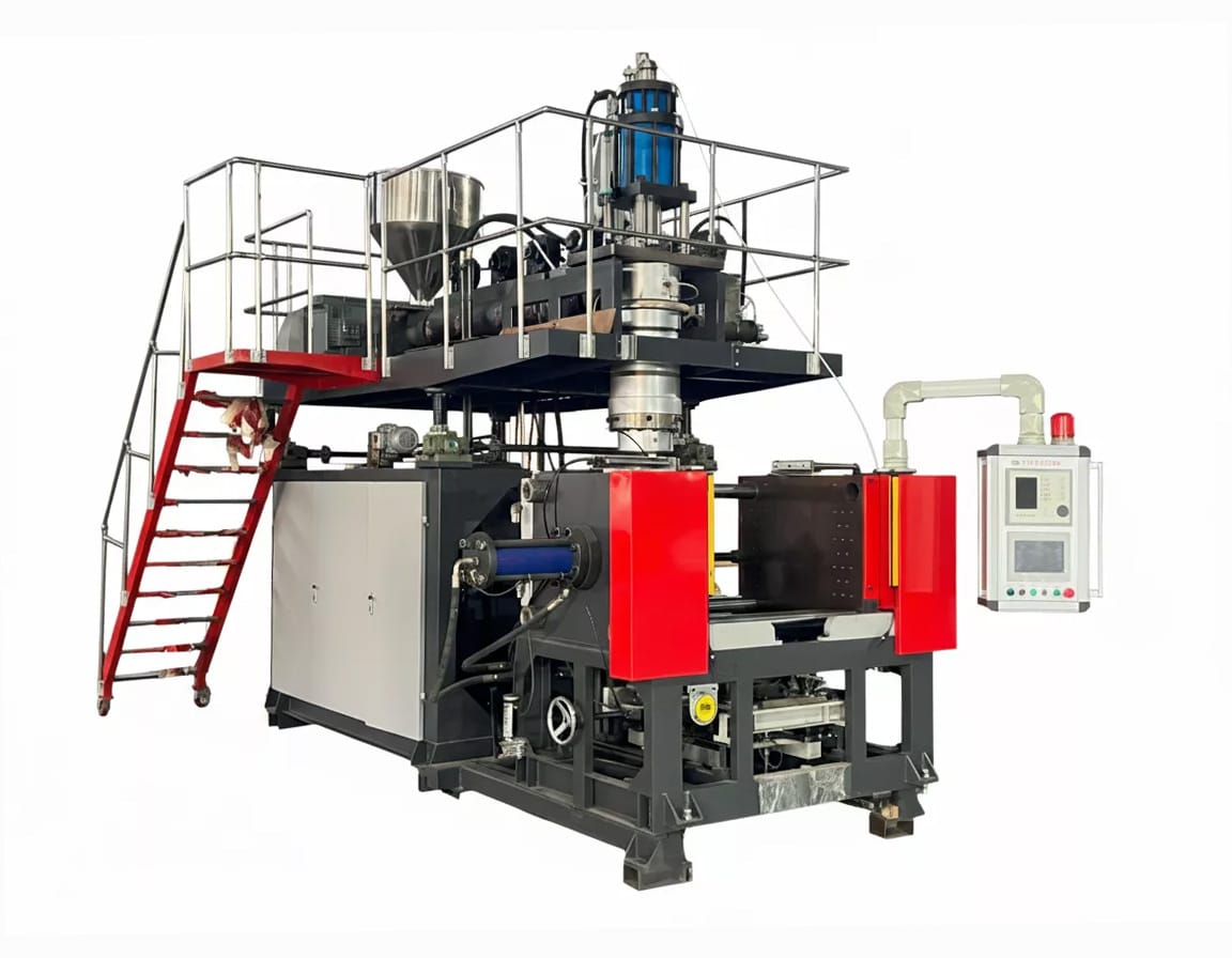
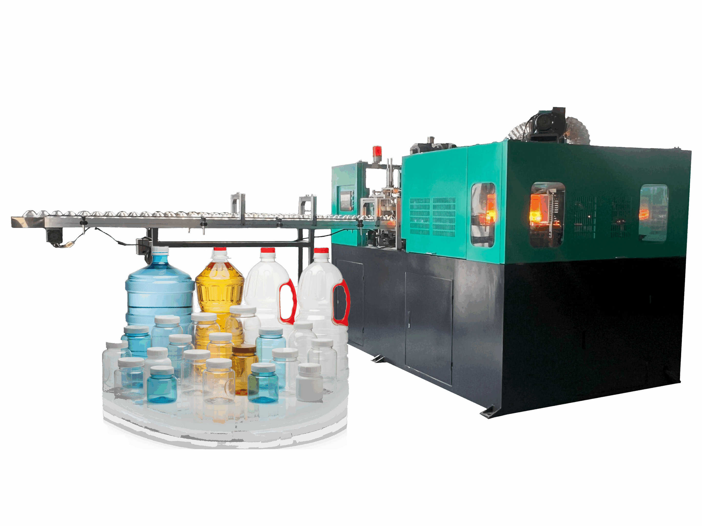
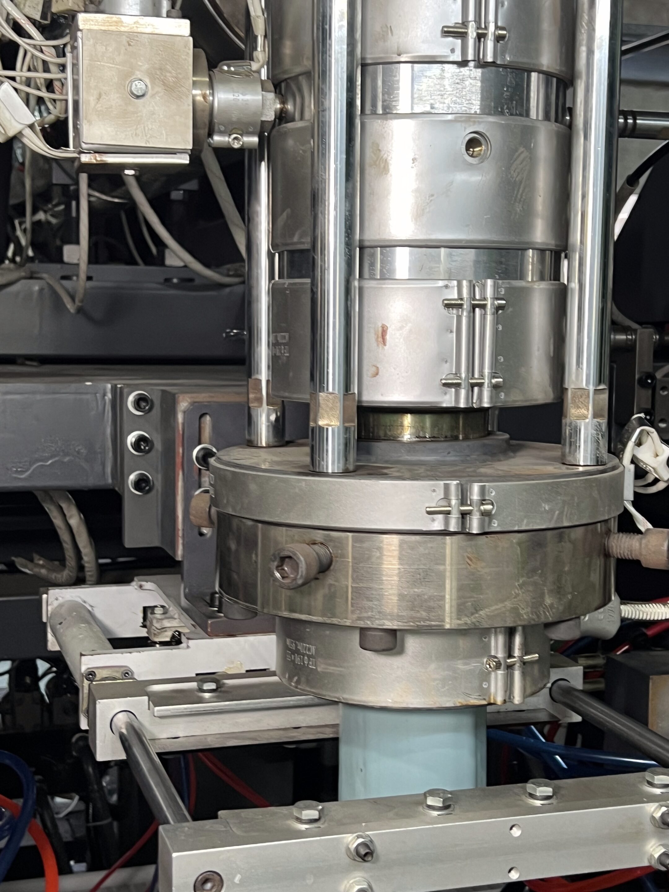
Machine: extrusion cetakan tiup or stretch blow molding base unit, with required options (parison control, servo drives).
Die head or preform path: die head, accumulators, or stretch blow oven and transfer where relevant.
Molds: bottle/jerry can molds, neck inserts, cavity sets, quick-change hardware.
Downstream: deflashing/trimmer, leak tester, conveyors, bottle grabbers, vision checks if needed.
Utilities: chiller, air compressor (low/high pressure for stretch blow), dryers, transformers.
Site: rigging, installation, anchoring, safety guarding, CE/UKCA docs if berlaku.
Services: commissioning, operator training, spare parts kit, lubrication, first-year maintenance plan.
Avoid
Don’t ignore commissioning ramp-up. First-month output is rarely at nameplate, and scrap is higher until recipes and trims are dialed in. Plan a ramp curve and extra resin for startup waste.
Tools
Vendor quote breakdown: ask for line-item pricing for machine, tooling, downstream, utilities, install, and services. No lump sums.
Commissioning checklist: power-up, heater soak, parison profile, mold alignment, leak tester calibration, quality sign-off, training hours completed.
Hasil
You get a full landed CapEx for each option, apples-to-apples. That makes it easy to compare extrusion vs. stretch blow setups by total investment, not just brochure price.
Visual
Show a simple bar chart with stacked components: machine, die head/oven, molds, downstream, utilities, site, services. One stack per option so differences are obvious at a glance.
Model Energy and Utilities per Good Bottle

Bottom line: calculate real energy per good bottle by logging actual kWh/hr during production runs, then divide by good bottles per hour using true OEE and scrap, and add compressed air and cooling loads from utility data to get an all-in cost per SKU and an annualized utility cost forecast.
What to do
Measure line electricity kWh/hour during steady production for each SKU and format; use meter logs or EMS data, not nameplate kW, to capture real speed losses and stops.
Compute good bottles per hour from OEE: OEE=Availability×Performance×Quality, then Good UPH=Nameplate UPH×OEE for each SKU and shift condition.
Convert to kWh per good bottle: kWh/baik=kWh/jam (jalur)Botol baik/jam menggunakan jendela data periode OEE aktual, bukan rata-rata harian.
Tambahkan energi udara bertekanan: perkirakan kWh kompresor dari log atau kinerja spesifik kWh/m³ dan konsumsi udara per botol SKU; kalikan harga listrik dengan kWh/m³ untuk mendapatkan €/m³ dan konversikan ke biaya per botol.
Tambahkan kWh pendingin/chiller: gunakan daya chiller dan siklus tugas selama proses SKU berjalan; alokasikan berdasarkan bagian beban panas jika chiller melayani banyak jalur.
Rumus
OEE: OEE=Availability×Performance×Quality; Ketersediaan =Waktu ProsesWaktu Terencana; Kinerja =Waktu Siklus Ideal×Jumlah TotalWaktu Proses; Kualitas =Jumlah BaikJumlah Total.
Botol baik per jam: Good UPH=Nameplate UPH×OEE atau langsung dari pencacah: Jumlah BaikJam Proses.
Listrik per botol baik (proses): kWh/baikproses=kWh/jam (terukur)UPH Baik.
Energi udara bertekanan: jika tanpa meteran, gunakan kinerja spesifik: kWh/m³=kWh Kompresorm³ yang Disalurkan; energi per botol =Udara (m³/botol)×kWh/m³; biaya per m³ ≈ harga listrik × kWh/m³.
Energi pendinginan: kWh/baikpendingin=kW Chiller×Bagian Beban×Siklus TugasUPH Baik untuk jendela proses SKU.
Sumber data
Lembar tarif: ambil biaya energi (€/kWh), biaya permintaan (€/kW), jendela TOU, pajak; hitung tarif campuran per shift untuk konversi biaya.
Biaya permintaan: perkirakan puncak kW bulanan dari data interval; alokasikan ke biaya SKU menggunakan jam puncak bersamaan atau kW rata-rata selama proses SKU berjalan untuk menghindari pengurangan biaya sebenarnya.
Kalkulator utilitas dan EMS: gunakan untuk mengekspor kWh dan kW per interval 15 menit untuk jalur, ruang kompresor, dan chiller agar selaras dengan jumlah produksi.
Avoid
Jangan gunakan kW nameplate atau kecepatan teoretis tanpa OEE dan scrap terukur; hal ini akan mengurangi kWh per botol baik dan mengabaikan waktu menganggur serta penghentian kecil.
Jangan rata-ratakan antar hari dengan pergantian; hitung per jendela SKU dengan kondisi proses yang stabil untuk penyebut yang bersih.
Target keluaran
Laporkan per SKU: proses kWh/baik, udara bertekanan kWh/baik, pendinginan kWh/baik, dan total biaya energi per botol baik menggunakan tarif campuran yang berlaku dan alokasi permintaan.
Akumulasikan ke biaya utilitas tahunan: kalikan biaya energi per-SKU dengan perkiraan volume botol baik tahunan; tambahkan biaya tambahan perawatan/modal udara bertekanan dan pendingin jika membangun total beban utilitas, biasanya patokan peningkatan ~10–25%.
Visual
Diagram perhitungan: kWh/jam (jalur) → bagi dengan UPH Baik (dari OEE) → kWh/baik (proses) → tambahkan Udara kWh/baik → tambahkan Pendinginan kWh/baik → Total kWh/baik → × tarif → Biaya energi/baik → × volume tahunan → Biaya utilitas tahunan.
Kuantifikasi Waktu Operasi, OEE, dan Biaya Downtime
Tujuannya sederhana: tetapkan Ketersediaan, Kinerja, dan Kualitas nyata dari data proses, lalu berikan harga wajar untuk setiap jam yang hilang sehingga downtime muncul dalam uang, bukan hanya menit. Ketika ketiga bagian OEE tersebut didasarkan pada log—bukan perkiraan—perencanaan dan keputusan ROI berhenti melenceng, karena keluaran dan kerugian dikuantifikasi dengan cara yang sama setiap kali.
Actions
Tetapkan tiga faktor OEE per SKU dan shift dari proses stabil terbaru: Ketersediaan = Waktu Proses / Waktu Terencana; Kinerja = (Waktu Siklus Ideal × Jumlah Total) / Waktu Proses; Kualitas = Jumlah Baik / Jumlah Total; OEE = A × P × Q.
Harga produksi yang hilang per jam menggunakan UPH Baik × margin kontribusi per unit; tambahkan tenaga kerja menganggur, overhead yang terpakai selama penghentian, dan biaya perbaikan tipikal dari catatan perawatan dan SLA untuk menghindari penghitungan yang kurang.
Build a downtime ledger: list top loss reasons (breakdown, changeover, resin change, block/starve), count events, average duration, and total hours to forecast annual exposure and target fixes with real numbers.
Avoid
Avoid assuming 90%+ OEE without logging changeovers, minor stops, and resin variability; these hit Availability and Performance more than most teams expect.
Avoid using nameplate speed for Performance; use ideal cycle time and actual counts over run time so slow cycles and micro‑stops are captured.
Tools
Maintenance logs for MTBF/MTTR, typical fault durations, and parts consumed; these feed Availability and cost-of-repair lines in the ledger.
Service SLAs and parts lead times to model extended MTTR windows and the probability of longer outages when spares aren’t on hand.
Hasil
A per‑SKU sheet with Availability, Performance, Quality, OEE, Good UPH, and monetized downtime exposure, rolled up by line and plant for annual downtime cost and OEE‑backed output.
A ranked list of loss buckets showing where time and money leak, justifying SMED workshops, preventive work, or resin SOPs with clear capacity and cash impact.
Rumus
OEE: OEE=Availability×Performance×Quality.
Availability: Run TimePlanned Production Time; Performance: Ideal Cycle Time×Total CountRun Time; Quality: GoodTotal.
Downtime cost per event: (Good UPH×Contribution Margin)×Downtime Hours+Idle Labor+Overheads+Repairs.
Visual
OEE pie chart with three slices—Availability, Performance, Quality—summing to 100%, annotated with top availability losses like changeovers and breakdowns from the downtime ledger.
Calculate Scrap and Material Losses
This step is about turning every gram of waste into a clear cost so material losses stop hiding in averages and assumptions, especially in cetakan tiup where flash, start‑ups, and thickness variation add up fast. When scrap is logged by type and multiplied by real resin prices and part weights, it becomes a simple per‑bottle and annual number that’s easy to track and improve.
Actions
Log start‑up scrap: count and weigh rejects during heat‑up and mold start, then tag by SKU, mold, and resin grade so the cost can be tied to specific conditions and shift patterns.
Track steady‑state rejects: use the basic scrap rate formula—Scrap Rate = Scrap Quantity / Total Production—to quantify ongoing defects and convert to mass using SKU weight specs for accurate resin costs.
Capture flash and regrind loop: record flash mass per cycle and actual refeed percentage; note that blow molding routinely generates large regrind volumes and properties can shift versus virgin, affecting usable blend ratios and yield.
Multiply by resin price: compute cost for each scrap bucket as Scrap Mass × Resin Price; report both cost per good bottle and annual cost using SKU volumes and negotiated resin rates.
Avoid
Don’t ignore parison control and wall thickness programs—poor control drives overweight parts and higher reject rates; modern parison control evens thickness and can cut part weight materially while improving quality.
Don’t assume all regrind behaves like virgin; particle size and fines change bulk density and processing, impacting flow, stability, and defect rates if unmanaged.
Tools
SKU weight specs: use target weight and tolerance to convert counts to kilograms for precise scrap costing and to flag overweight trends that burn resin silently.
Parison control settings and mold data: correlate thickness profiles, head programs, and mold cavitation with scrap spikes to pinpoint where control changes reduce loss without hurting strength.
Hasil
Clear metrics: scrap cost per year and per good bottle by SKU, broken into start‑up, steady‑state, and flash/regrind categories so actions have obvious ROI and accountability.
Weight optimization: evidence that better parison control reduces average part weight and rejects, improving yield and lowering resin spend at the same time.
Rumus
Scrap rate by count: Scrap Rate=Scrap UnitsTotal Units and by mass: Scrap Rate=Scrap MassTotal Material Mass for periods or runs by SKU.
Scrap cost per good bottle: Cost/good=∑(Scrap Massi×Resin Price)Good Units with buckets for start‑up, steady‑state, and flash/regrind to show contributions.
Annual scrap cost: Annual Cost=Cost/good×Annual Good Units using forecast volumes to tie improvements to budget targets.
Example levers
Tighten parison profiles to reduce top‑to‑bottom thinning and overweight compensation, yielding more uniform walls and lower average part mass at spec.
Improve regrind quality by controlling particle size and removing fines to stabilize feed density and melt, which reduces steady‑state defects from flow variability.
Visual
Before/after scrap trendline: plot scrap rate or scrap kg per 10,000 bottles by week, annotating the date parison control adjustments were applied to show weight and reject reductions over time.
Labor, Changeovers, and Automation
This step turns people time and setup time into a clean cost per good bottle, then shows how automation and SMED reduce both without sacrificing quality checks. The idea is to define who touches the cell, how long changeovers actually take, and how often they happen—then price the lost hours and the labor that keeps running even when the line is stopped.
Actions
Define the staffing plan per shift: operators on the cell, material handling, and QC touches; use time studies or standard work to capture minutes per loop for inspection, pack-out, and rework so labor per unit is grounded in observed cycles.
Quantify changeovers: measure setup time from last good of SKU A to first good of SKU B, including tool/mold swaps, purging, parameter dialing, and verification; log frequency per week to forecast total setup hours.
Map automation options inline: note quick-change kits, preset recipes, tool carts, and automated stations such as inline deflashing and leak test that can reduce handling and QC touches without bottlenecking the line.
Avoid
Don’t forget start-up waste after each change—those first-off rejects are part of the setup window and should be costed along with lost time, not treated as “free” scrap.
Don’t assume a nominal staffing level covers QC; if leak test or deflashing is manual today, count those touches explicitly or justify automation that removes them from the labor denominator.
Rumus
Direct labor cost per good bottle: Labor/good=Direct labor hours (run + setup)Good units×Loaded wage rate where “run + setup” includes QC touches and documented changeover time.
Annual changeover loss hours: Setup hours/year=Avg setup hours/event×Events/year; monetize with Cost/hour=Good UPH×contribution margin+idle labor + overhead for capacity and cash impact.
Tools
Time studies and standard work: video and time the full setup and operator cycles; separate internal work (machine stopped) vs external work (machine running) to convert internal tasks to external per SMED.
Quick-change and inline stations: evaluate preset tooling, staged carts, and inline deflashing/leak test so changeovers shrink and QC becomes 100% automated without extra headcount or speed loss.
Hasil
A per‑SKU labor cost per good bottle that includes operators, QC, and setup allocation, plus an annualized changeover loss line item tied to frequency and duration.
A prioritized list of SMED and automation levers that free capacity and remove manual QC touches, improving OEE availability and stabilizing throughput without new headcount.
Visual
Cell layout diagram: show operator positions, quick‑change staging, and automated stations (deflash, leak test) on the flow, highlighting which QC touches are eliminated and which setup steps move external under SMED.
Maintenance, Spares, and Reliability
This step turns reliability into a budget line: plan the parts and PMs that will definitely be needed, price the time it takes to recover from failures, and hold critical spares on‑site where lead times would otherwise turn small issues into long outages. With MTBF/MTTR and a realistic PM schedule, years 2–5 costs stop being a surprise because both planned spend and risk‑adjusted downtime are modeled upfront.
Actions
Budget planned parts and PM labor: list PM tasks and intervals, attach parts kits and hours, and calendarize them to get a yearly parts-and-labor budget by asset and line.
Price MTTR and service response: use failure logs to estimate MTBF and MTTR, then price each failure using lost output per hour plus repair labor; include service SLA response lags that extend downtime windows.
Plan critical spares on‑site: run a criticality and lead‑time screen (ABC) to decide what to stock; set reorder points and record carrying cost so the stock vs. downtime trade‑off is explicit.
Avoid
Don’t underestimate years 2–5: wear parts, oil/filters, seals, hoses, sensors, heaters, valves, and drives stack up after warranty; budget replacements on the OEM cycle, not wishful thinking.
Don’t ignore lead times: long‑lead electronics and custom tooling should be stocked or dual‑sourced; otherwise MTTR balloons from hours to weeks despite good technicians.
Tools
PM schedule: reliability‑centered mix of preventive and condition‑based tasks with defined intervals and feedback loops to adjust frequencies as data improves.
Parts list and BOM: item master with cost, lead time, alternates, and ABC class to drive min/max and reorder points in the CMMS/EAM system.
Remote diagnostics: enable faster triage and first‑time‑fix by having telemetry and remote support in SLAs to shrink effective MTTR.
Rumus
MTBF: MTBF=Uptime HoursFailure Count; MTTR: MTTR=Repair Downtime HoursFailure Count for each asset or line family.
Availability from reliability: A=MTBFMTBF+MTTR; tie A back to OEE to see the impact of maintenance on output.
Risk‑adjusted downtime cost/year: ∑i(Failuresi/year)×MTTRi×Cost/hour, where Cost/hour includes lost margin, labor, and overhead for the line.
Hasil
A two‑part budget: 1) annual planned maintenance (parts and labor by PM interval) and 2) risk‑adjusted unplanned downtime cost from MTBF/MTTR and SLA assumptions.
Stocked critical spares with reorder points and carrying costs, reducing risk of long outages while making the capital tied in inventory transparent and purposeful.
Visual
Gantt of PM intervals: plot monthly/quarterly tasks per asset with parts kits and hour estimates; overlay failure‑based tasks as conditional bands to show where CBM signals would trigger additional work.
Finance, Depreciation, and Compare Alternatives
This step rolls financing, depreciation, and residual value into the true cost per good bottle and then compares machines head‑to‑head on cost/bottle, payback, and IRR—not just sticker CapEx. The idea is to translate OEE‑backed output and operating costs into cash flows, then use standard finance metrics so the better choice is obvious and defensible.
Actions
Add financing cost: include interest from loans or lease payments in the annual cash flows; for leases, use the payment schedule; for loans, include principal outlay and interest expense timing.
Set a depreciation schedule and residual value: choose tax depreciation (e.g., MACRS under GDS/ADS) or book straight‑line, and include expected resale value at end of horizon to reduce net cost of ownership in the model.
Compute cost per good bottle: allocate annual fixed costs (finance, depreciation, insurance) over OEE‑backed good units, then add variable costs (energy, labor, scrap, maintenance) to get all‑in cost/bottle by SKU.
Avoid
Don’t pick on CapEx alone; compare total cost/bottle and capital efficiency over time, because higher‑efficiency equipment often wins once output and operating costs are normalized.
Jangan abaikan payback dan IRR; ini menunjukkan waktu hingga impas dan pengembalian keseluruhan versus tingkat penghalang, serta memberikan penalti terhadap opsi dengan arus kas awal yang ringan atau ekor yang berat.
Tools
Payback dan IRR di spreadsheet: masukkan arus kas inkremental antara Mesin A dan B; gunakan fungsi IRR/NPV untuk mendapatkan payback dan IRR, dan tabel sensitivitas untuk menguji asumsi OEE, kWh/unit baik, tenaga kerja, dan scrap.
Rumus
IRR: selesaikan 0=CF0+∑t=1nCFt(1+IRR)t dengan alat IRR/NPV spreadsheet untuk kecepatan perhitungan praktis.
Biaya per botol: Biaya/unit baik=Biaya tahunan tetapUnit baik+Biaya variabel/unit baik, di mana biaya tetap termasuk depresiasi dan pembiayaan serta biaya variabel termasuk energi, tenaga kerja, scrap, perawatan.
Payback: nilai terkecil t di mana arus kas kumulatif berubah menjadi non-negatif ketika membandingkan opsi yang disukai versus baseline atau Mesin A versus B.
Hasil
Perbandingan berdampingan Mesin A vs. B yang menunjukkan biaya/botol, payback, dan IRR; pemenangnya harus memiliki biaya/botol lebih rendah dan payback yang dapat diterima pada atau di dalam horizon target dengan IRR di atas tingkat penghalang.
Visual dengan tabel atau dua batang untuk selisih biaya/botol, membuat keunggulan kapasitas dan biaya operasi mudah dijelaskan kepada keuangan dan operasi bersama-sama.
Tips bonus / langkah lanjutan
Minta data kWh per botol baik dan OEE untuk SKU sejenis dari vendor; waktu siklus saja menyesatkan tanpa memasukkan kerugian nyata.
Validasi asumsi dengan referensi pabrik atau uji coba singkat bila memungkinkan untuk mengurangi risiko model dalam input OEE dan scrap sebelum berkomitmen.
Model musiman: bulan lebih panas dapat meningkatkan beban chiller dan tingkat cacat, menggeser kWh/unit baik dan scrap; cantumkan ini dalam arus kas bulanan jika tarif energi dibedakan berdasarkan waktu dalam setahun.
Pertimbangkan variabilitas rHDPE/PCR; kontrol suhu dan parison yang lebih ketat sering meningkatkan hasil dan menstabilkan berat, yang mengurangi biaya scrap dan energi per unit baik.
Visual
Bagan sederhana A vs. B: dua batang untuk biaya per botol, diberi anotasi dengan unit baik berbasis OEE yang digunakan dalam penyebut; sertakan tabel kecil di bawahnya dengan payback dan IRR sehingga keputusan bergantung pada finansial lengkap, bukan hanya CapEx.
Kesimpulan
Harga pokok rendah dapat menyembunyikan energi, scrap, dan downtime yang lebih tinggi. Dengan mendefinisikan ruang lingkup, memuat OEE nyata, dan mengonversi semuanya menjadi biaya per botol baik, Anda membuat perbandingan lebih bersih dan keputusan payback lebih cepat. Gunakan lembar 8-langkah, lalu minta data vendor dalam format sama untuk membandingkan seperti-dengan-seperti. Ingin kalkulator TCO siap pakai yang disesuaikan untuk *ekstrusi blow molding* dan pergantian SKU? Minta spreadsheet-nya, dan saya akan membagikannya.
tautan eksternal
Rumus OEE yang Perlu Anda Ketahui — Lineview Solutions
https://lineview.com/en/oee-formulas-you-need-to-know/Overall Equipment Effectiveness (OEE) — MPDV USA
https://us.mpdv.com/industry-4-0/smart-factory-glossary/overall-equipment-effectiveness-oeeEfisiensi Energi Udara Terkompresi (PDF) — CED Engineering
https://www.cedengineering.com/userfiles/M06-013%20-%20Compressed%20Air%20Energy%20Efficiency%20-%20US.pdfBerapa biaya 1 m³ udara terkompresi? — WRS Energie
https://wrs-energie.de/en/how-much-does-1m%C2%B3-of-compressed-air-cost/Interval 15 Menit dalam Manajemen Energi — CLOU Global
https://clouglobal.com/from-theory-to-practice-the-struggles-of-implementing-15-minute-intervals-in-energy-management/Pengukuran Daya Sistem Pemantauan Energi (PDF) — IEA 4E
https://www.iea-4e.org/wp-content/uploads/2021/01/APPENDIX_A_Guidance_document_for_energy_measurement_of_EMS.pdfMTTR, MTBF, MTTD, MTTF: Panduan Komparatif — Squadcast
https://www.squadcast.com/blog/system-reliability-metrics-a-comparative-guide-to-mttr-mtbf-mttd-and-mttfSingle Minute Exchange of Die (SMED) — Six Sigma (6sigma.us)
https://www.6sigma.us/lean-tools/single-minute-exchange-of-die-smed/SMED dijelaskan: Kurangi waktu pergantian — Kaizen Institute
https://kaizen.com/insights/smed-reduce-changeover-boost-efficiency/Modified Accelerated Cost Recovery System (MACRS) — Investopedia (dengan referensi IRS Pub. 946)
https://www.investopedia.com/terms/m/macrs.asp


0 Komentar