

Introducción
“Cheapest machine” often turns into the most expensive line after year two. Energy spikes, scrap drift, and downtime eat margins fast. In this guide, I show a simple, practical way to model Total Cost of Ownership (TCO) for an extrusion blow molding machine—so you judge by cost per good bottle, not sticker price. You’ll map the big cost buckets, pressure-test key assumptions, and compare two machines apples-to-apples. Short, clear steps. Actionable checks. Use it before the next RFQ.
What You’ll Need
Last 12 months’ run hours, SKU mix, scrap %, and good bottles/hour per SKU.
Local electricity tariff and demand charges; compressed air and chiller specs.
Resin price range (virgin HDPE, rHDPE/PCR), typical gram weights.
Maintenance logs: planned/unplanned stops, parts spend, MTTR.
Quotes for machines, tooling, auxiliaries, installation, and servicio terms.
Define Scope and Time Horizon

Pick a clear window: 5–10 years is enough to cover one or two major upgrades and show total cost, not just the purchase price. Shorter than 5 years hides maintenance and energy costs. Longer than 10 years gets fuzzy because product lines, materials, and labor rules change.
Actions
Choose a time horizon: 5, 7, or 10 years. Keep it consistent across options.
List SKUs you’ll run: sizes, resins (like HDPE or PET), and bottle/jerry can families. Note annual volume and seasonality.
Define shifts: 1–3 shifts per day, days per week, planned uptime, and maintenance stops. Convert that into annual available hours.
Estimate growth: base case, conservative, and stretch. Tie growth to real triggers like a new customer contract or recycled material requirements.
Avoid
Don’t compare “cycle time” across machines without SKU mix and changeover rules. A fast cycle on paper can lose in real life if changeovers are frequent, scrap spikes on certain resins, or the mold set is limited.
Tools
Use one spreadsheet with three tabs:
Assumptions: time horizon, SKUs, shifts, uptime, growth, resin type.
Costs: CapEx, molds, utilities, labor per shift, maintenance, spare parts, training.
Results: output per year, cost per bottle, total cost of ownership, sensitivity cases.
Outcome
You end up with a clean boundary: what’s inside the model and what’s not. That keeps debates focused on inputs, not opinions.
Visual
Show one simple timeline: CapEx in Year 0, then OpEx bars (energy, labor, maintenance) for each year. Add markers where growth or SKU changes kick in.
Capture CapEx and Tooling
Build the CapEx list from the clamp to the conveyor. The goal is a true “landed” cost, not just the base machine. Keep it simple, but complete.
Actions
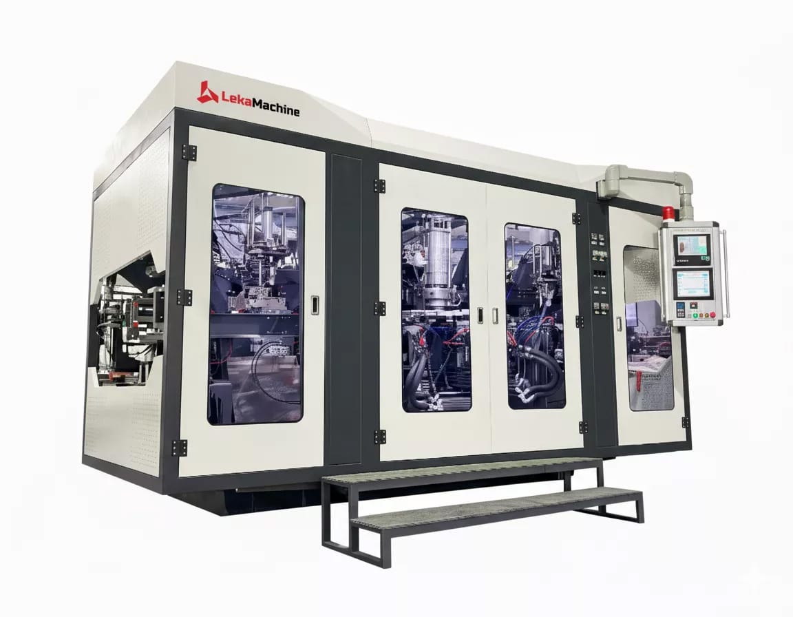
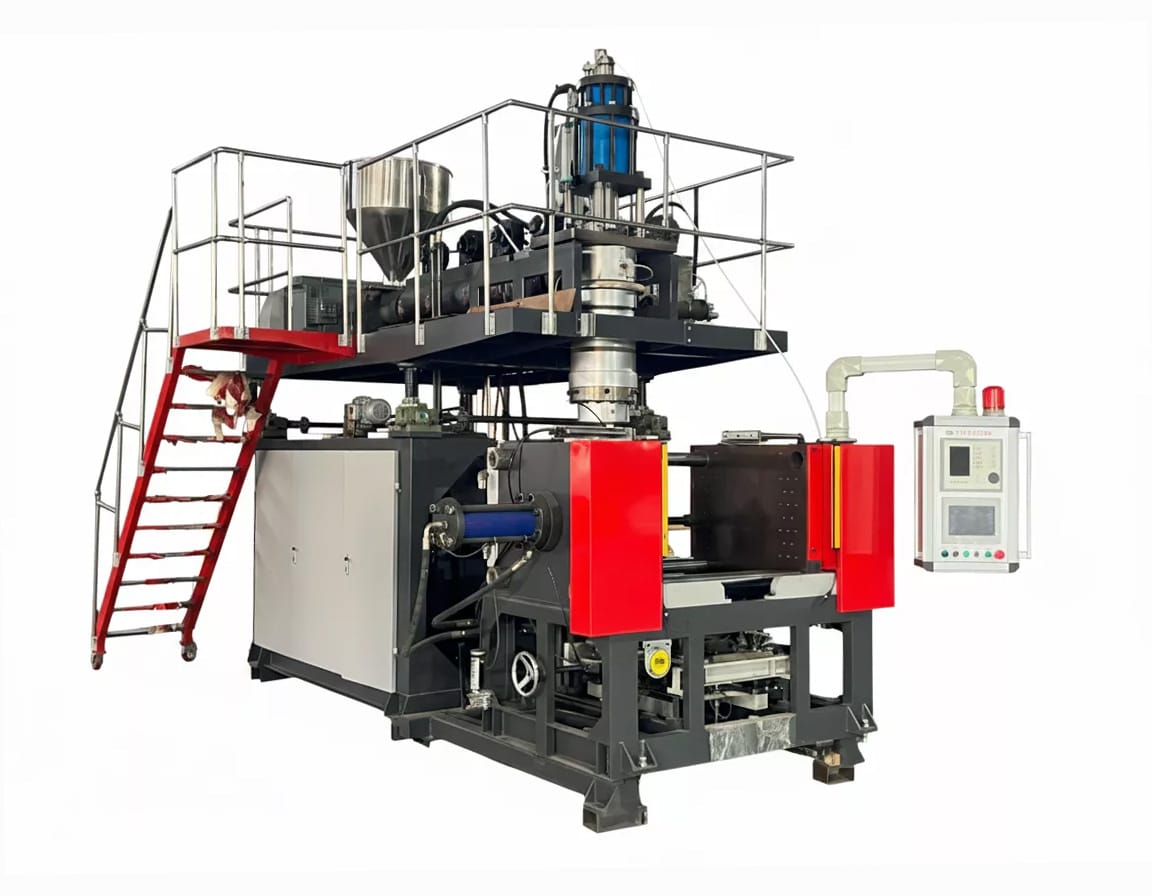
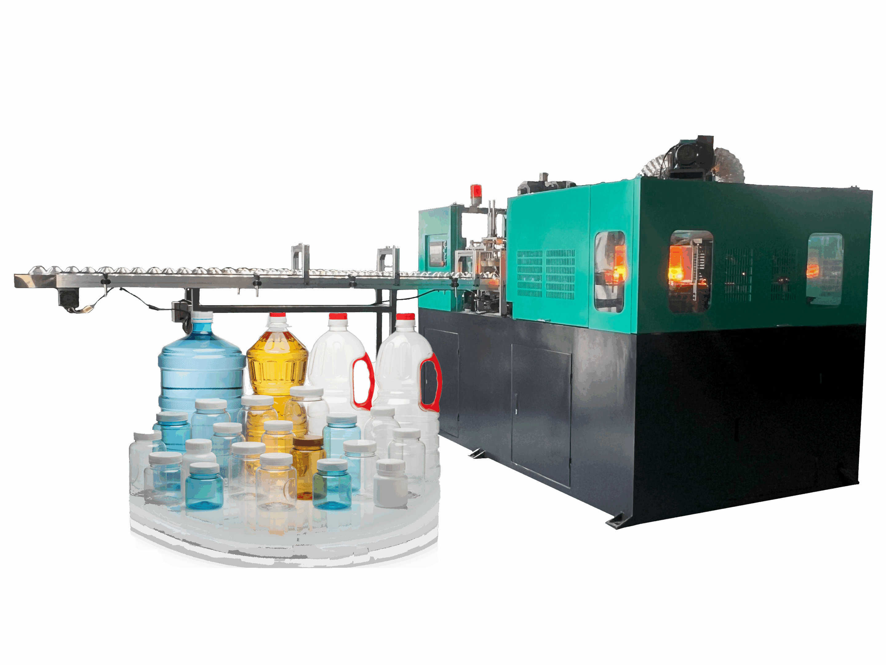
Machine: extrusion moldeo por soplado or stretch blow molding base unit, with required options (parison control, servo drives).
Die head or preform path: die head, accumulators, or el moldeo por estirado-soplado oven and transfer where relevant.
Molds: bottle/jerry can molds, neck inserts, cavity sets, quick-change hardware.
Downstream: deflashing/trimmer, leak tester, conveyors, bottle grabbers, vision checks if needed.
Utilities: chiller, air compressor (low/high pressure for el moldeo por estirado-soplado), dryers, transformers.
Site: rigging, installation, anchoring, safety guarding, CE/UKCA docs if sea aplicable..
Services: commissioning, operator training, spare parts kit, lubrication, first-year maintenance plan.
Avoid
Don’t ignore commissioning ramp-up. First-month output is rarely at nameplate, and scrap is higher until recipes and trims are dialed in. Plan a ramp curve and extra resin for startup waste.
Tools
Vendor quote breakdown: ask for line-item pricing for machine, tooling, downstream, utilities, install, and services. No lump sums.
Commissioning checklist: power-up, heater soak, parison profile, mold alignment, leak tester calibration, quality sign-off, training hours completed.
Outcome
You get a full landed CapEx for each option, apples-to-apples. That makes it easy to compare extrusion vs. stretch blow setups by total investment, not just brochure price.
Visual
Show a simple bar chart with stacked components: machine, die head/oven, molds, downstream, utilities, site, services. One stack per option so differences are obvious at a glance.
Model Energy and Utilities per Good Bottle

Bottom line: calculate real energy per good bottle by logging actual kWh/hr during production runs, then divide by good bottles per hour using true OEE and scrap, and add compressed air and cooling loads from utility data to get an all-in cost per SKU and an annualized utility cost forecast.
What to do
Measure line electricity kWh/hour during steady production for each SKU and format; use meter logs or EMS data, not nameplate kW, to capture real speed losses and stops.
Compute good bottles per hour from OEE: OEE=Availability×Performance×Quality, then Good UPH=Nameplate UPH×OEE for each SKU and shift condition.
Convert to kWh per good bottle: kWh/good=kWh/hr (line)Good bottles/hr using actual OEE-period data windows, not daily averages.
Add compressed air energy: estimate compressor kWh from logs or specific performance kWh/m3 and SKU’s air consumption per bottle; multiply electricity price by kWh/m3 to get €/m³ and convert to per-bottle cost.
Add cooling/chiller kWh: use chiller power and duty cycle during that SKU’s run; apportion by heat load share if the chiller serves multiple lines.
Formulas
OEE: OEE=Availability×Performance×Quality; Availability =Run TimePlanned Time; Performance =Ideal Cycle Time×Total CountRun Time; Quality =Good CountTotal Count.
Good bottles per hour: Good UPH=Nameplate UPH×OEE or directly from counters: Good CountRun Hours.
Electricity per good bottle (process): kWh/goodprocess=kWh/hr (measured)Good UPH.
Compressed air energy: if meterless, use specific performance: kWh/m3=Compressor kWhDelivered m3; energy per bottle =Air (m3/bottle)×kWh/m3; cost per m³ ≈ electricity price × kWh/m3.
Cooling energy: kWh/goodcool=Chiller kW×Load Share×DutyGood UPH for the SKU run window.
Data sources
Tariff sheet: pull energy charge (€/kWh), demand charge (€/kW), TOU windows, taxes; compute blended rate per shift for cost conversion.
Demand charges: estimate monthly peak kW from interval data; allocate to SKU cost using coincident peak hours or average kW during the SKU run to avoid understating true cost.
Utility calculators and EMS: use to export kWh and kW by 15‑min interval for the line, compressor room, and chiller to align with production counts.
Avoid
Don’t use nameplate kW or theoretical speed without measured OEE and scrap; it will understate kWh per good bottle and miss idle and minor stops.
Don’t average across days with changeovers; compute per-SKU windows with stable run conditions for clean denominators.
Output targets
Report per SKU: process kWh/good, compressed air kWh/good, cooling kWh/good, and total energy cost per good bottle using the applicable blended tariff and demand allocation.
Roll up to annual utility cost: multiply per-SKU energy cost by annual good bottle volume forecast; add compressed air and cooling maintenance/capital adders if building total utility burden, typically ~10–25% uplift benchmarks.
Visual
Calculation diagram: kWh/hr (line) → divide by Good UPH (from OEE) → kWh/good (process) → add Air kWh/good → add Cooling kWh/good → Total kWh/good → × tariff → Energy cost/good → × annual volume → Annual utility cost.
Quantify Uptime, OEE, and Downtime Cost
The goal here is simple: lock in real Availability, Performance, and Quality from run data, then put a fair price on each lost hour so downtime shows up in money, not just minutes. When those three OEE pieces are grounded in logs—not guesses—planning and ROI decisions stop drifting, because output and loss are quantified the same way every time.
Actions
Set the three OEE factors by SKU and shift from recent stable runs: Availability = Run Time / Planned Time; Performance = (Ideal Cycle Time × Total Count) / Run Time; Quality = Good / Total; OEE = A × P × Q.
Price lost production per hour using Good UPH × contribution margin per unit; add idle labor, overhead burned during stops, and typical repair costs from maintenance records and SLAs to avoid undercounting.
Build a downtime ledger: list top loss reasons (breakdown, changeover, resin change, block/starve), count events, average duration, and total hours to forecast annual exposure and target fixes with real numbers.
Avoid
Avoid assuming 90%+ OEE without logging changeovers, minor stops, and resin variability; these hit Availability and Performance more than most teams expect.
Avoid using nameplate speed for Performance; use ideal cycle time and actual counts over run time so slow cycles and micro‑stops are captured.
Tools
Maintenance logs for MTBF/MTTR, typical fault durations, and parts consumed; these feed Availability and cost-of-repair lines in the ledger.
Service SLAs and parts lead times to model extended MTTR windows and the probability of longer outages when spares aren’t on hand.
Outcome
A per‑SKU sheet with Availability, Performance, Quality, OEE, Good UPH, and monetized downtime exposure, rolled up by line and plant for annual downtime cost and OEE‑backed output.
A ranked list of loss buckets showing where time and money leak, justifying SMED workshops, preventive work, or resin SOPs with clear capacity and cash impact.
Formulas
OEE: OEE=Availability×Performance×Quality.
Availability: Run TimePlanned Production Time; Performance: Ideal Cycle Time×Total CountRun Time; Quality: GoodTotal.
Downtime cost per event: (Good UPH×Contribution Margin)×Downtime Hours+Idle Labor+Overheads+Repairs.
Visual
OEE pie chart with three slices—Availability, Performance, Quality—summing to 100%, annotated with top availability losses like changeovers and breakdowns from the downtime ledger.
Calculate Scrap and Material Losses
This step is about turning every gram of waste into a clear cost so material losses stop hiding in averages and assumptions, especially in moldeo por soplado where flash, start‑ups, and thickness variation add up fast. When scrap is logged by type and multiplied by real resin prices and part weights, it becomes a simple per‑bottle and annual number that’s easy to track and improve.
Actions
Log start‑up scrap: count and weigh rejects during heat‑up and mold start, then tag by SKU, mold, and resin grade so the cost can be tied to specific conditions and shift patterns.
Track steady‑state rejects: use the basic scrap rate formula—Scrap Rate = Scrap Quantity / Total Production—to quantify ongoing defects and convert to mass using SKU weight specs for accurate resin costs.
Capture flash and regrind loop: record flash mass per cycle and actual refeed percentage; note that blow molding routinely generates large regrind volumes and properties can shift versus virgin, affecting usable blend ratios and yield.
Multiply by resin price: compute cost for each scrap bucket as Scrap Mass × Resin Price; report both cost per good bottle and annual cost using SKU volumes and negotiated resin rates.
Avoid
Don’t ignore parison control and wall thickness programs—poor control drives overweight parts and higher reject rates; modern parison control evens thickness and can cut part weight materially while improving quality.
Don’t assume all regrind behaves like virgin; particle size and fines change bulk density and processing, impacting flow, stability, and defect rates if unmanaged.
Tools
SKU weight specs: use target weight and tolerance to convert counts to kilograms for precise scrap costing and to flag overweight trends that burn resin silently.
Parison control settings and mold data: correlate thickness profiles, head programs, and mold cavitation with scrap spikes to pinpoint where control changes reduce loss without hurting strength.
Outcome
Clear metrics: scrap cost per year and per good bottle by SKU, broken into start‑up, steady‑state, and flash/regrind categories so actions have obvious ROI and accountability.
Weight optimization: evidence that better parison control reduces average part weight and rejects, improving yield and lowering resin spend at the same time.
Formulas
Scrap rate by count: Scrap Rate=Scrap UnitsTotal Units and by mass: Scrap Rate=Scrap MassTotal Material Mass for periods or runs by SKU.
Scrap cost per good bottle: Cost/good=∑(Scrap Massi×Resin Price)Good Units with buckets for start‑up, steady‑state, and flash/regrind to show contributions.
Annual scrap cost: Annual Cost=Cost/good×Annual Good Units using forecast volumes to tie improvements to budget targets.
Example levers
Tighten parison profiles to reduce top‑to‑bottom thinning and overweight compensation, yielding more uniform walls and lower average part mass at spec.
Improve regrind quality by controlling particle size and removing fines to stabilize feed density and melt, which reduces steady‑state defects from flow variability.
Visual
Before/after scrap trendline: plot scrap rate or scrap kg per 10,000 bottles by week, annotating the date parison control adjustments were applied to show weight and reject reductions over time.
Labor, Changeovers, and Automation
This step turns people time and setup time into a clean cost per good bottle, then shows how automation and SMED reduce both without sacrificing quality checks. The idea is to define who touches the cell, how long changeovers actually take, and how often they happen—then price the lost hours and the labor that keeps running even when the line is stopped.
Actions
Define the staffing plan per shift: operators on the cell, material handling, and QC touches; use time studies or standard work to capture minutes per loop for inspection, pack-out, and rework so labor per unit is grounded in observed cycles.
Quantify changeovers: measure setup time from last good of SKU A to first good of SKU B, including tool/mold swaps, purging, parameter dialing, and verification; log frequency per week to forecast total setup hours.
Map automation options inline: note quick-change kits, preset recipes, tool carts, and automated stations such as inline deflashing and leak test that can reduce handling and QC touches without bottlenecking the line.
Avoid
Don’t forget start-up waste after each change—those first-off rejects are part of the setup window and should be costed along with lost time, not treated as “free” scrap.
Don’t assume a nominal staffing level covers QC; if leak test or deflashing is manual today, count those touches explicitly or justify automation that removes them from the labor denominator.
Formulas
Direct labor cost per good bottle: Labor/good=Direct labor hours (run + setup)Good units×Loaded wage rate where “run + setup” includes QC touches and documented changeover time.
Annual changeover loss hours: Setup hours/year=Avg setup hours/event×Events/year; monetize with Cost/hour=Good UPH×contribution margin+idle labor + overhead for capacity and cash impact.
Tools
Time studies and standard work: video and time the full setup and operator cycles; separate internal work (machine stopped) vs external work (machine running) to convert internal tasks to external per SMED.
Quick-change and inline stations: evaluate preset tooling, staged carts, and inline deflashing/leak test so changeovers shrink and QC becomes 100% automated without extra headcount or speed loss.
Outcome
A per‑SKU labor cost per good bottle that includes operators, QC, and setup allocation, plus an annualized changeover loss line item tied to frequency and duration.
A prioritized list of SMED and automation levers that free capacity and remove manual QC touches, improving OEE availability and stabilizing throughput without new headcount.
Visual
Cell layout diagram: show operator positions, quick‑change staging, and automated stations (deflash, leak test) on the flow, highlighting which QC touches are eliminated and which setup steps move external under SMED.
Maintenance, Spares, and Reliability
This step turns reliability into a budget line: plan the parts and PMs that will definitely be needed, price the time it takes to recover from failures, and hold critical spares on‑site where lead times would otherwise turn small issues into long outages. With MTBF/MTTR and a realistic PM schedule, years 2–5 costs stop being a surprise because both planned spend and risk‑adjusted downtime are modeled upfront.
Actions
Budget planned parts and PM labor: list PM tasks and intervals, attach parts kits and hours, and calendarize them to get a yearly parts-and-labor budget by asset and line.
Price MTTR and service response: use failure logs to estimate MTBF and MTTR, then price each failure using lost output per hour plus repair labor; include service SLA response lags that extend downtime windows.
Plan critical spares on‑site: run a criticality and lead‑time screen (ABC) to decide what to stock; set reorder points and record carrying cost so the stock vs. downtime trade‑off is explicit.
Avoid
Don’t underestimate years 2–5: wear parts, oil/filters, seals, hoses, sensors, heaters, valves, and drives stack up after warranty; budget replacements on the OEM cycle, not wishful thinking.
Don’t ignore lead times: long‑lead electronics and custom tooling should be stocked or dual‑sourced; otherwise MTTR balloons from hours to weeks despite good technicians.
Tools
PM schedule: reliability‑centered mix of preventive and condition‑based tasks with defined intervals and feedback loops to adjust frequencies as data improves.
Parts list and BOM: item master with cost, lead time, alternates, and ABC class to drive min/max and reorder points in the CMMS/EAM system.
Remote diagnostics: enable faster triage and first‑time‑fix by having telemetry and remote support in SLAs to shrink effective MTTR.
Formulas
MTBF: MTBF=Uptime HoursFailure Count; MTTR: MTTR=Repair Downtime HoursFailure Count for each asset or line family.
Availability from reliability: A=MTBFMTBF+MTTR; tie A back to OEE to see the impact of maintenance on output.
Risk‑adjusted downtime cost/year: ∑i(Failuresi/year)×MTTRi×Cost/hour, where Cost/hour includes lost margin, labor, and overhead for the line.
Outcome
A two‑part budget: 1) annual planned maintenance (parts and labor by PM interval) and 2) risk‑adjusted unplanned downtime cost from MTBF/MTTR and SLA assumptions.
Stocked critical spares with reorder points and carrying costs, reducing risk of long outages while making the capital tied in inventory transparent and purposeful.
Visual
Gantt of PM intervals: plot monthly/quarterly tasks per asset with parts kits and hour estimates; overlay failure‑based tasks as conditional bands to show where CBM signals would trigger additional work.
Finance, Depreciation, and Compare Alternatives
This step rolls financing, depreciation, and residual value into the true cost per good bottle and then compares machines head‑to‑head on cost/bottle, payback, and IRR—not just sticker CapEx. The idea is to translate OEE‑backed output and operating costs into cash flows, then use standard finance metrics so the better choice is obvious and defensible.
Actions
Add financing cost: include interest from loans or lease payments in the annual cash flows; for leases, use the payment schedule; for loans, include principal outlay and interest expense timing.
Set a depreciation schedule and residual value: choose tax depreciation (e.g., MACRS under GDS/ADS) or book straight‑line, and include expected resale value at end of horizon to reduce net cost of ownership in the model.
Compute cost per good bottle: allocate annual fixed costs (finance, depreciation, insurance) over OEE‑backed good units, then add variable costs (energy, labor, scrap, maintenance) to get all‑in cost/bottle by SKU.
Avoid
Don’t pick on CapEx alone; compare total cost/bottle and capital efficiency over time, because higher‑efficiency equipment often wins once output and operating costs are normalized.
Don’t ignore payback and IRR; these show time to breakeven and overall return versus the hurdle rate, and they penalize options with light early cash flows or heavy tails.
Tools
Spreadsheet payback and IRR: enter incremental cash flows between Machine A and B; use IRR/NPV functions to get payback and IRR, and sensitivity tables to test OEE, kWh/good, labor, and scrap assumptions.
Formulas
IRR: solve 0=CF0+∑t=1nCFt(1+IRR)t with spreadsheet IRR/NPV tools for practical calculation speed.
Cost per bottle: Cost/good=Fixed annual costsGood units+Variable cost/good, where fixed includes depreciation and financing and variable includes energy, labor, scrap, maintenance.
Payback: smallest t where cumulative cash flow turns non‑negative when comparing the preferred option vs. baseline or Machine A vs. B.
Outcome
Side‑by‑side Machine A vs. B showing cost/bottle, payback, and IRR; the winner should have the lower cost/bottle and acceptable payback at or inside the target horizon with IRR above the hurdle.
A visual with a table or two bars for cost/bottle difference, making the capacity and operating‑cost advantages easy to explain to finance and operations together.
Bonus tips / advanced moves
Ask vendors for kWh per good bottle and OEE on similar SKUs; cycle time alone is misleading without real losses included.
Validate assumptions with a factory reference or short trial run when possible to reduce model risk in OEE and scrap inputs before committing.
Model seasonality: hotter months can raise chiller load and defect rates, shifting kWh/good and scrap; reflect this in monthly cash flows if energy tariffs are time‑of‑year differentiated.
Consider rHDPE/PCR variability; tighter temperature and parison control often improves yield and stabilizes weight, which reduces scrap cost and energy per good.
Visual
Simple A vs. B chart: two bars for cost per bottle, annotated with the OEE‑backed good units used in the denominator; keep a small table beneath with payback and IRR so decisions hinge on complete financials, not just CapEx.
Conclusión
A low sticker price can hide higher energy, scrap, and downtime. By defining scope, loading real OEE, and converting everything to cost per good bottle, you make cleaner comparisons and faster payback decisions. Use the 8-step sheet, then request vendor data in the same format to compare apples-to-apples. Want a ready-to-use TCO calculator tailored for moldeo por soplado por extrusión and SKU changeovers? Ask for the spreadsheet, and I’ll share it.
external link
OEE Formulas You Need to Know — Lineview Solutions
https://lineview.com/en/oee-formulas-you-need-to-know/Overall Equipment Effectiveness (OEE) — MPDV USA
https://us.mpdv.com/industry-4-0/smart-factory-glossary/overall-equipment-effectiveness-oeeCompressed Air Energy Efficiency (PDF) — CED Engineering
https://www.cedengineering.com/userfiles/M06-013%20-%20Compressed%20Air%20Energy%20Efficiency%20-%20US.pdfHow much does 1 m³ of compressed air cost? — WRS Energie
https://wrs-energie.de/en/how-much-does-1m%C2%B3-of-compressed-air-cost/15-Minute Intervals in Energy Management — CLOU Global
https://clouglobal.com/from-theory-to-practice-the-struggles-of-implementing-15-minute-intervals-in-energy-management/Power Measurement of Energy Monitoring Systems (PDF) — IEA 4E
https://www.iea-4e.org/wp-content/uploads/2021/01/APPENDIX_A_Guidance_document_for_energy_measurement_of_EMS.pdfMTTR, MTBF, MTTD, MTTF: Comparative Guide — Squadcast
https://www.squadcast.com/blog/system-reliability-metrics-a-comparative-guide-to-mttr-mtbf-mttd-and-mttfSingle Minute Exchange of Die (SMED) — Six Sigma (6sigma.us)
https://www.6sigma.us/lean-tools/single-minute-exchange-of-die-smed/SMED explained: Reduce changeover time — Kaizen Institute
https://kaizen.com/insights/smed-reduce-changeover-boost-efficiency/Modified Accelerated Cost Recovery System (MACRS) — Investopedia (with IRS Pub. 946 references)
https://www.investopedia.com/terms/m/macrs.asp


0 Comentarios